Using dplyr and foreach to read in multiple data sets from disk
I had a student (Jack Fogliasso) bring me a problem from a Microbiology lab where they are trying to identify bacteria using lasers. One of the items they wanted to understand was the absorption rates of different wavelengths. So they have a machine to do the lasering and it reads out a text file that of course has a ton of meta data in it, is semi-colon delimited, and there’s one file per trial. So not the standard situation that one might encounter in a basic applied statistics class.
Jack and I talked about automation and reproducibility and how R is great for tasks like this, and he got to work. What is shown below is an effective use of dplyr and to read in a data set from disk, do some processing, and create a visualization. This process can be expanded to any number of files thanks to the efficient looping of foreach, and the combination of dplyr and ggplot2 can accommodate different file names, such as for different new bacteria.
System setup
This example uses the ggplot2, dplyr and foreach packages.
knitr::opts_chunk$set(echo = TRUE, warning=FALSE, message=FALSE)
library(ggplot2)
library(dplyr)
library(foreach)
Data import
Read in the data for the three experimental trials.
- get all .txt files in the working directory and put into a list.
list_files <- list.files(pattern = ".txt", full.names = TRUE)
list_files
## [1] "./Ec1.txt" "./Ec2.txt" "./Ec3.txt"- Use the
%do%function in theforeachpackage to efficiently loop over all items in the list. This read in the data usingread.delim, turns it into a data frame, so that we can add the file name to the data set before combining each data set usingrbind(stacking or concatonating).
eColi <- foreach(i=1:length(list_files), .combine=rbind) %do% {
            read.delim(list_files[[i]], skip=66, sep=";") %>%
            data.frame() %>%
            mutate(file=gsub(".txt", "", list_files[[i]]))# add an identifier to index each trial
}
head(eColi)## Pixel Wavelength Dark Reference Raw.data..1 Dark.Subtracted..1 X.TR..1
## 1 0 349.84 1161.60 1266.60 1257.96 96.36 91.7714
## 2 1 350.27 1160.72 1263.56 1258.04 97.32 94.6324
## 3 2 350.71 1161.20 1262.84 1259.56 98.36 96.7729
## 4 3 351.14 1158.96 1264.04 1256.76 97.80 93.0719
## 5 4 351.58 1150.24 1259.64 1252.12 101.88 93.1261
## 6 5 352.01 1144.08 1256.92 1243.72 99.64 88.3020
## Absorbance..1 Raw.data..2 Dark.Subtracted..2 X.TR..2 Absorbance..2
## 1 0.0373 0 0 0 0
## 2 0.0240 0 0 0 0
## 3 0.0142 0 0 0 0
## 4 0.0312 0 0 0 0
## 5 0.0309 0 0 0 0
## 6 0.0540 0 0 0 0
## Raw.data..3 Dark.Subtracted..3 X.TR..3 Absorbance..3 Lamp.FitCurve
## 1 0 0 0 0 0
## 2 0 0 0 0 0
## 3 0 0 0 0 0
## 4 0 0 0 0 0
## 5 0 0 0 0 0
## 6 0 0 0 0 0
## Irradiance.Ratio Irradiance_1.W.cm.2.nm. Irradiance_2.W.cm.2.nm.
## 1 0 NA 0
## 2 0 NA 0
## 3 0 NA 0
## 4 0 NA 0
## 5 0 NA 0
## 6 0 NA 0
## Irradiance_3.W.cm.2.nm. file
## 1 0 ./Ec1
## 2 0 ./Ec1
## 3 0 ./Ec1
## 4 0 ./Ec1
## 5 0 ./Ec1
## 6 0 ./Ec1- Shorten the names to something reasonable.
names(eColi)[c(5:16,19:21)] <- paste0(rep(c("raw", "dark", "X", "abs", "irr"),3), 1:3)
names(eColi)
## [1] "Pixel" "Wavelength" "Dark" "Reference"
## [5] "raw1" "dark2" "X3" "abs1"
## [9] "irr2" "raw3" "dark1" "X2"
## [13] "abs3" "irr1" "raw2" "dark3"
## [17] "Lamp.FitCurve" "Irradiance.Ratio" "X1" "abs2"
## [21] "irr3" "file"Data Processing
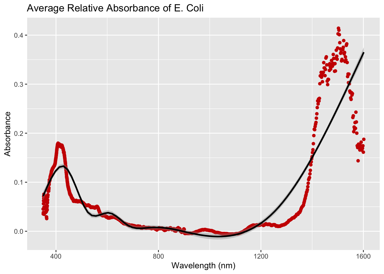
Create the average absorbance of the 3 trials per wave length.
eColi_abs <- eColi %>% group_by(Wavelength) %>% summarise(avgRelAbs = mean(abs1))
head(eColi_abs)## # A tibble: 6 x 2
## Wavelength avgRelAbs
## <dbl> <dbl>
## 1 350. 0.0453
## 2 350. 0.0353
## 3 351. 0.0382
## 4 351. 0.0562
## 5 352. 0.0621
## 6 352. 0.0713Analyzing
Plot the average relative absorbance for the E. coli.
ggplot(eColi_abs, aes(x=Wavelength, y=avgRelAbs)) +
              geom_point(color="#CC0000") + geom_smooth(color="black") +
              labs(title="Average Relative Absorbance of E. Coli",
                   x="Wavelength (nm)", y="Absorbance")